Whether and to what extent age is a prevalent factor in the technical job market are questions that are frequently raised in press articles, blog posts, and discussion boards. The usual—but by no means sole—concern is that tech companies discriminate against older workers in favor of younger ones. The sources of this tendency are multi-faceted. First, there is the long-standing historical precedent recognized in 1967 when the Age Discrimination in Employment Act was enacted in which it became federal law to prohibit discrimination against people 40 years or older in employment matters. Thus, contemporary debates about ageism in tech should recognize that such discrimination is neither recent nor peculiar to the tech industry. Clearly there was a bias against older workers long before the modern tech industry and occupations like software engineering even existed.

Yet there is another cultural aspect to ageism that is indeed endemic to tech. Unlike enduring professions such as law, medicine, and finance, there is a mystique about tech which suggests that it—even moreso than mathematics according to Hardy’s famous quote—is a “young man’s game”. The landscape of today’s highly successful tech companies is replete with examples of founders who vaulted into the public sphere at a very early age: Gates and Allen, Brin and Page, Jobs and Wozniak, Mark Zuckerberg, Elon Musk, and so on. In popular culture, the ‘start-up’ is almost universally characterized with imagery of boy geniuses casually revolutionizing the world in between gulps of Red Bull and games of foosball. Each new cohort is introduced to the myth by films like Wargames (Generation X), Hackers (Generation Y), and The Social Network (Generation Zero). As long ago as 1992, Neal Stephenson observed in his epic Snow Crash, “Software development, like professional sports, has a way of making thirty-year-old men feel decrepit.”

In an oft-maligned quote, Mark Zuckerberg once remarked to a roomful of hopeful young startup founders that “young people are just smarter”. In context, it’s not actually the bald-faced pronouncement of ageism that it has been taken to assume. He was responding to the anxiety that young founders were feeling, that they were not experienced enough to make the right decisions in building their products. Zuck was attempting to boost their confidence by reminding them that youth has some innate advantages and that their instincts could in fact serve them very well. Still, it can be disconcerting to say the least to hear such words being casually tossed about as youthful inspiration. Why is every class of Y Combinator’s Startup School filled with fresh-faced twenty-one year olds? Are they in fact smarter than their predecessors? Is software really a young man’s game and noone wants to invest in a company founded by 40 year olds? Or, perhaps more cynically, are the fresh recruits of startup school merely selected for by gambler-investors who are more than eager to cheaply acquire the surplus labor of willing smart young hackers who’ve been sold on the idea that their hundred hour work weeks for Ramen money are going to change the world?

The examples enshrined in Microsoft, Google, Facebook, et. al. reflect a gold-rush culture in tech the underlying current of which suggests that if you’re any good you’ll be rich by the time you’re 30. I think this is a very important and under-studied psychological aspect of ageism in tech that affects both young and old alike: “Why is this 50 year old software engineer on the job market… he must not be very good if he’s not uber-rich yet!” I am certain that this mindset affects hiring decisions in tech. When a company is comparing a smart 20 year old with a smart 50 year old, the younger one simply has a lot more potential energy—she could be the next Big Thing! A larger proportion of the older engineer’s potential has already been converted to kinetic energy, so there’s a smaller chance that the 10x lottery ticket will pay off. Let’s hire the young one… she’s a “digital native” after all.

Anecdotally, I have been fortunate not to have personally experienced ageism thus far in my career. At least, I don’t think I have—clearly, one of the pernicious aspects of discrimination is that one can often not be certain of having been subjected to it. Nor do I personally know of anyone who has been discriminated against based on their age. Maybe I’m just not old enough yet and it is simply a matter of time. The closest I have come to age discrimination was once when I was trying to explain some data analysis I was doing to a young Ruby boot-camp graduate who remarked to me, “R? Only old people use R!”

It was a joke of course and I certainly don’t equate this with actual discrimination. Ageism is a serious matter because it can affect the livelihood and life chances of real people in very significant ways. Does ageism exist in tech? I’m certain it does, given the amount of attention it receives and the numerous examples that surface from time to time. But what do we mean by ageism and how could we observe instances of it? The typical manifestation is in hiring practices—that young workers will be favored over older ones. Ageism may also be implicated in layoffs, where older workers are let go disproportionately more often than younger ones. It may also be evident in salary comparisons—if ageism is more prevalent in tech occupations, then one would expect to see a shallow earnings curve as age progresses in comparison to other occupations. There are of course many other less tangible but nonetheless real manifestations of ageism. Older workers may be passed over for promotions, may be assigned to less prestigious tasks, or their opinions may not be valued as highly in meetings. Because it is such a multi-faceted issue, it would be foolish to assume that any single dataset could be used to prove or disprove that ageism exists.

In this analysis I am interested in examining whether ageism can be detected in aggregate statistics of the working population. Given the need to examine motivations for behavior and employment practices, determining when an instance of age discrimination has occurred is far more suited to case law than data analysis. So I have no illusions that I will convince anyone one way or another with incontrovertible proof. Consider this more an introductory exploration of publically available data brought to bear on questions of age in the technical occupation market of the United States.

The American Community Survey is a block-stratified random sample of US households conducted year-round by the Census Bureau since 2000. It replaced the Census long-form questionnaire and serves as the most comprehensive demographic dataset of US households and residents. Highly detailed tables can be generated directly on the Census’s American Factfinder website. Through its Public-Use Microdata Samples, the Census Bureau makes available yearly extracts of the ACS which anyone can use to conduct analyses of their own. Each year, the ACS PUMS dataset consists of a 1% national random sample of the entire US population.

The most recent ACS release is for the calendar year 2015. One of the easiest ways to obtain ACS datasets is from the IPUMS project of the Minnesota Population Center at the University of Minnesota. IPUMS offers a convenient extract system with a wealth of documentation about the available samples and variables. In addition, many IPUMS variables are presented with consistent coding schemes across samples, making multi-year analyses much easier than working with the raw PUMS datasets provided by the Census Bureau.

Since I am a strong believer in reproducible research, I’m making all of the code used in this analysis available for your scrutiny. Whether you are interested solely in replicating these findings, or would like to use them as a springboard for your own custom analysis, I hope you will find the code straightforward. The analysis was conducted in R and the code is available here: acs2015_age-and-tech.R.txt.

Before we begin, let’s try to enumerate some hypotheses about what we may expect to find in our dataset. If ageism is a significant factor in technical occupations, how might it be manifest in broad statistics about the population? A logical place to start is with the age distribution of technical occupations. If tech truly is a young man’s game, then we may expect to find a disproportionate concentration of tech workers among younger age cohorts as compared to the broader working population or other specific occupations. Next, we can examine the earnings curve: as age, and presumably experience, progresses, do older workers in tech gain earning power at similar levels as seen in other occupations? Regarding the employment rate, we can see whether older tech workers are unemployed or out of the labor force at higher rates than younger ones. Perhaps ageism is not so much a consequence of being in a technical occupation, but is rather driven by the tech industry. Thus, we can look at age, income, and employment in the tech industry vs. other industries. We can then go further and segment technical occupations within technical companies to see if there are large-scale indications of ageism in such segments.

It is important to understand the limitations of our analysis given our choice of dataset. While the ACS dataset does provide a rich source of demographic data, in many ways it is insufficient for an in-depth study of occupational status. For instance, while we know each respondent’s occupation, as well as other basic demographic detail such as their educational attainment and degree field, we do not know the number of years experience they have in that occupation. We also do not know specific job titles. Thus, we can only rely on age as a rough proxy for experience and must assume that the distribution of experience levels is fairly consistent across occupations.

Now, before we dive into the data, try to answer this question: what do you think is the average age of software developers in the US? Would you say 25? 35? Would you be surprised to learn that the average age is in fact 41? For comparison, across all occupations, the average age for all workers 16 years or older is 42. For those of you who, reasonably, are suspicious of averages, the median age is 39 for software developers compared to 42 for all workers. Clearly there is a slight skew on the younger side but it by no means paints a picture of software developers as being all fresh grads.

Before continuing further, let’s take a moment to study the IPUMS variables we will be using in this analysis. It is extremely important to understand the data collection methodology, the question texts and instructions, and the coding schemes of all the variables to ensure that we are interpreting the results accurately. The list below contains a brief description of and links to the IPUMS documentation for all the variables involved in the analysis. The dataset we are using is the American Community Survey 2015 sample. For more information about the ACS, there is a great deal of background information and technical reports on the Census Bureau’s project page.

• PERWT. The number of persons in the US population represented by each person in the sample. This is the most important variable in the entire dataset so I wanted to mention it first. The ACS is not a true random sample—it is stratified by Census blocks to provide a representative sample of households—so you will not get accurate statistics unless you apply appropriate weights. For person-level analysis, you should use PERWT, and for household level analysis, you should use HHWT. Note also that for any calculation involving variance you should scale PERWT to sum to the sample count (which is 3,147,005 in the 2015 ACS). You can run into all kinds of problems with inflated variance from artificial population weights. Many statistical functions can handle re-scaling of weight variables automatically. For example, in R, the wtd.stats set of functions in the Hmisc package include a normwt argument which if set equal to TRUE will rescale the weights to sum to the sample size instead of the population size. You can also do this explicitly by creating a new variable, which is the approach I have taken in the sample code.
• AGE. Person’s age at last birthday. In the 2015 ACS sample, the range is 0 to 97.
• OCC. The person’s primary occupation, for all persons 16 years or older who had worked within the previous five years. The respondent describes each person’s job in their own words, and the Census Bureau assigns the response to an occupation category code. For the 2015 ACS, there are 479 occupation codes. For a description of the occupational coding scheme, see this link.
• IND. The type of industry in which the person was employed. This is also written in free-form and coded into one of 267 different industry codes. Here is a link to the industry classification codes.
• EMPSTAT. The current (prior week) employment status for each person. This indicates for all persons 16 years or older whether they were employed, unemployed, or out of the labor force—neither employed nor actively looking for work.
• WKSWORK2. The number of weeks worked in the prior 12 months, coded into convenient categories. Here, we typically filter on a value of 6 which is coded as 50 to 52 weeks (which is meant to include paid vacations and holidays). This is useful when we want to restrict the analysis to only those who worked year-round in the prior 12 months—for example, in income comparisons we don’t want to compare people who only worked 6 months with people who worked all 12 months.
• UHRSWORK. The usual number of hours worked per week in the prior 12 months. This is also used as a filter to include full-time workers as opposed to part-time. We use 35 or more hours per week as the definition of full-time.
  
• INCWAGE. Total pre-tax salary or wage earnings in the prior 12 months. Note that a value of 999999 is a code for a missing value and must be filtered out of any analysis. In addition, beware that values above the 99.5th percentile are top-coded as the mean of all such values in the person’s state of residence. There are many additional income related variables. We focus on INCWAGE because in this analysis we are concerned with earnings among workers in employer-employee settings, rather than, for example, business owners.

Now let’s explore the Census Bureau’s occupational coding scheme as used in the 2015 ACS. As noted above, respondents write in their own words a description of each person’s primary occupation. The Census standardizes this by coding the responses into one of 479 different occupation codes. Note that we don’t have access to the raw text entered by the respondents. Nor do we have any say in how the Census Bureau has coded each response. And even though there are 479 unique occupation codes, these have been designed to reflect the entire working economy of the US, and may not make as sharp of a distinction among certain technical positions. For example, there is no code specifically for Data Scientists (maybe next year) and there isn’t much visibility into how the Census Bureau would have mapped “Data Scientist” to an occupation code. That caveat aside, the most relevant “tech” occupations are clustered together in the range from 1005 to 1107. The table below reports the relevant occupation codes along with their description as provided by the Census Bureau, their unweighted count in the 2015 ACS, and the weighted count estimating the number of persons in the US having each as their primary occupation. Feel free to review the complete list of occupation codes and include additional codes in your own analysis.

OCC Code	Unweighted count	Weighted count	Label
1005	215	22,971	Computer and information research scientists
1006	5,416	552,870	Computer systems analysts
1007	712	71,627	Information security analysts
1010	4,989	508,834	Computer programmers
1020	12,657	1,302,041	Software developers, applications and systems software
1030	2,121	221,806	Web developers
1050	7,173	736,514	Computer support specialists
1060	1,346	129,397	Database Administrators
1105	2,360	232,037	Network and Computer Systems Administrators
1106	1,114	116,267	Computer network architects
1107	6,264	655,014	Computer occupations, all other

All together, these 11 occupation codes represent 4,549,378 people in the US, 2.4% of the population 16 years or older.

Age by occupation

Let’s explore the age distribution of these occupations, starting with the full working population for reference.

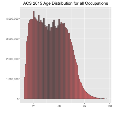
As noted above, both the mean and median age for the full working population is 42. This includes everyone 16 years and older who have worked at any point in the past 5 years. Let’s see what this age distribution looks like for each of the 11 technical occupations listed above. [My apologies to mobile viewers out there, I haven’t yet figured out the magical combination of arguments to ggplot2 to make these lattice plots look nice on all browsers.]

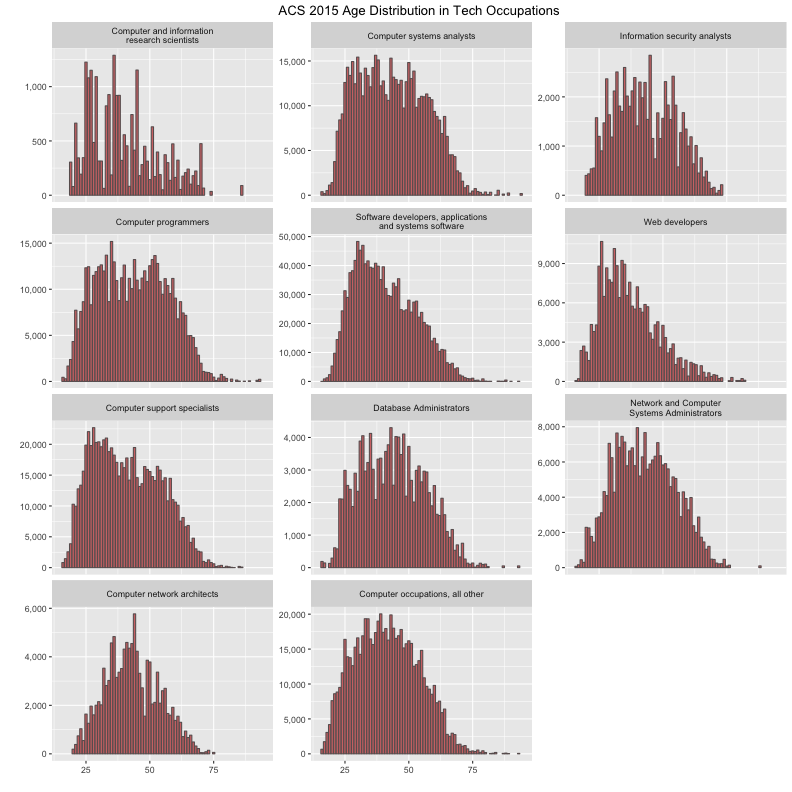
As we examine these plots, keep in mind the unweighted sample sizes for each occupation as listed in the table above. A few of them have very low sample sizes so the age distributions will be very spiky. For example, the first occupation “Computer and information research scientists” has a sample size of only 215. The most populous of these occupations, “Software developers, applications and systems software”, has a healthy sample size of 12,657 and represents a population count of 1,302,041. The age distribution for this occupation is roughly similar to the overall age distribution for all occupations, but there is somewhat of a skew toward younger ages. The most notable skew is among “Web developers”, where the mean age is 37.1 and the median is 35. Clearly this new-fangled web development thing is attracting a lot of young-uns.

When sorted by average age from youngest to oldest, Web developers ranks #43 out of all 479 occupations. It has a similar age distribution as Physical Therapist Assistants, Riggers, Childcare Workers, and Customer Service Representatives, but it is by no means among the occupations that skew the youngest. Lifeguards has a median age of just 19. Military crew members, Counter Attendants, Dancers and Choreographers, Cashiers, Athletes, and Food Preparation Workers are some additional examples of occupations where the median age is under 30.

Among technical occupations, Database Administrators has the oldest age skew, with an average age of 43.8. Computer programmers and Computer systems analysts have a similar age distribution. Occupations with similar age distributions include Cargo and Freight Agents, Dieticians and Nutritionists, Dental Hygienists, Pharmacists, and Railroad Conductors and Yardmasters. As far as all occupations are concerned, these rank roughly in the middle, very similar to the overall age distribution of the full working population. The occupations that skew oldest, with median ages around 55, include Motor Vehicle Operators, Embalmers and Funeral Attendants, Crossing Guards, Clergy, and Chief executives and legislators.

For reference, you can find the weighted population count, mean, and median age for all occupations in occ-age.html.

Income by age

Now let’s turn to income, as measured by the INCWAGE variable in the IPUMS dataset. Recall that this only includes salary and wage income earned over the past 12 months. In order to ensure that we have a consistent metric for each occupation, we will only include the subset of workers who were employed year-round (50-52 weeks in the prior 12 months) and usually worked full-time (35 or more hours per week). In addition, we will restrict the analysis to ages 18 to 65. First, let’s start with a reference for the entire population of full-time year-round workers in all occupations.

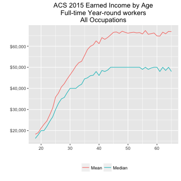
We have a couple of interesting asymptotic looking curves here, with rapid gains between 20 and 30, a somewhat slower but still strongly increasing trend in the 30s, until age 45 when both mean and median become basically flat from there on out. Now let’s see how these earnings curves look for out tech occupations.

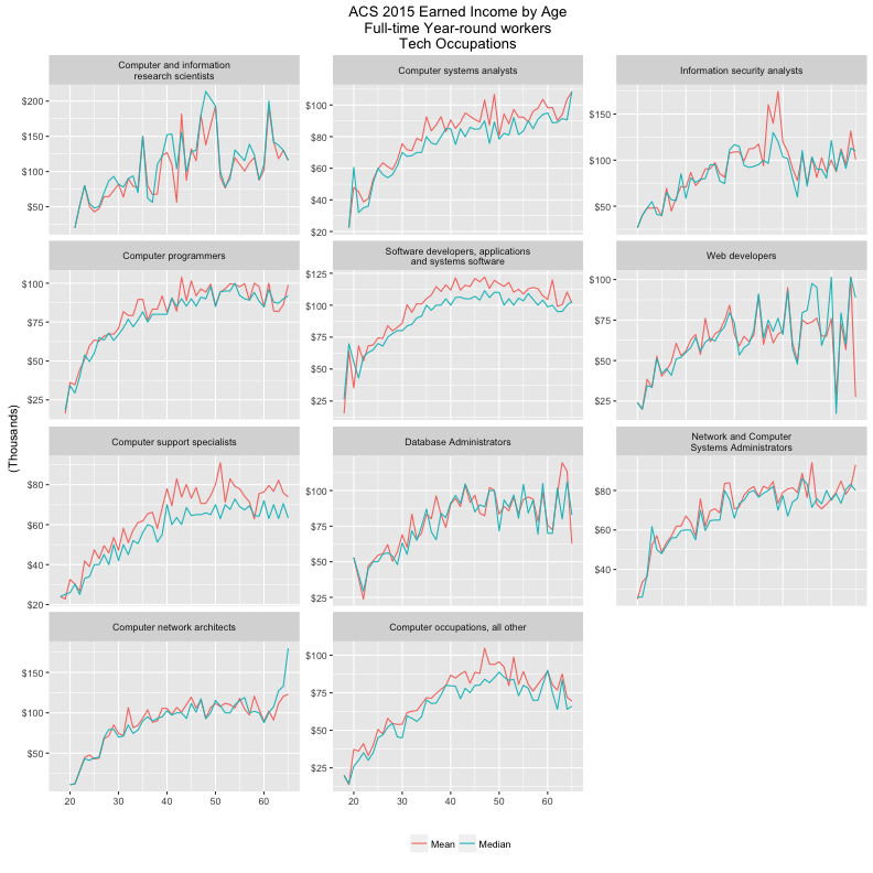
Again, for reference I’ve calculated the mean and median earnings for all occupations (full-time, year-round, but no age restrictions) available in occ-inc.html. This table is sorted by mean income from highest to lowest. Among all occupations, the mean earnings is $57,156 and the median is $42,000.

Software developers ranks #23 in the list of all occupations, with average earnings of $104,401 and median of $95,000. In fact, all of our tech occupations are well above average. Web developers has the lowest average earnings in our list—perhaps owing to the fact that it also has the youngest age skew—but even here the average is $62,148 and the median is $58,000.

The earnings curve for Software developers, the most populous of our tech occupations, behaves somewhat differently from the overall curve. While income peaks in the 40s, it begins to reverse course somewhat throughout the 50s to the point where developers in their late 50s are on average earning similarly to those in their late 30s. Hmmm, is this ageism? Of course it might be, but there could be a lot of other factors going on here. Keep in mind that we can only use age as a rough proxy for experience, as we don’t have any way of normalizing occupational experience levels across the age spectrum.

Let’s now cherry-pick some interesting occupations to use as comparisons. In professions like law, medicine, and finance, one would expect that age and experience would go hand in hand with higher marketability and thus more earning power. Below are the earnings curves by age for four of these professions all of which appear among the occupations with the highest overall income.

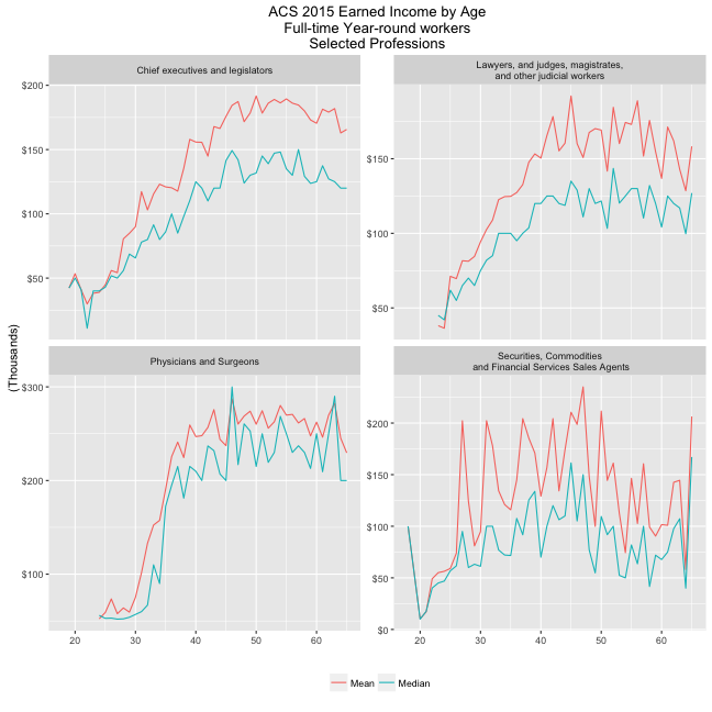
Lawyers and doctors both appear to reach their peak earnings power around 40, with both curves staying relatively flat throughout the 50s. On its face, this does not appear too different from our technical occupations. Among Chief executives and legislators, their income curve does not grow as quickly as the other professions, but it also peaks later, well into the 50s. The mean and median age for this occupation is 53, one of the oldest of all occupations. In finance, there’s much more variance than in other occupations, and not nearly as much earnings appreciation by age.

[Technical note: there was only one 22 year old Lawyer in the dataset and his or her reported income was above the topcode threshold. I excised this record from the dataset for better readability.]

Occupation by age

In the first section above, we look at the age distribution by occupation—that is, for all workers in a given occupation, what percentage is represented by each age. Another way to look at this is to flip the proportions around to consider the occupation distribution by age. For any given age, what percentage of workers are employed in a given occupation. Earlier we noted that the weighted total for our 11 selected technical occupations represents 2.4% of the population 16 years or older. If we consider the subset of the population aged 18 to 65 working full-time and year-round in the past 12 months, we find that our tech occupations account for 3.3% of this active subset of the working population. The plot below shows us, for each age, the percent of the active working population (full-time, year-round) who work in one of the 11 tech occupations.

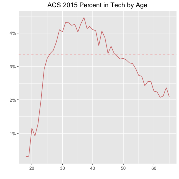
The dotted line is the reference point for the entire population, at 3.3%. Ages above this line are over-represented in tech, while those below are under-represented. Tech occupations are under-represented until age 26 at which point they become over-represented until age 48 when they dip below the average again. This may reflect movement from individual contributor to management roles, but we are unable to explore this hypothesis with the ACS dataset.

Employment status by age

The EMPSTAT variable records whether each person was employed, unemployed, or out of the labor force in the previous week. If one of the potential manifestations of ageism is that older workers have a more difficult time remaining employed, we may be able to detect that by examining the percentage of those in tech occupations whose status is employed. Among workers 18-65 in all occupations, 83% were employed in the prior week. For those in tech occupations, the percent employed is 91%. Below we can see the employment curve by age.

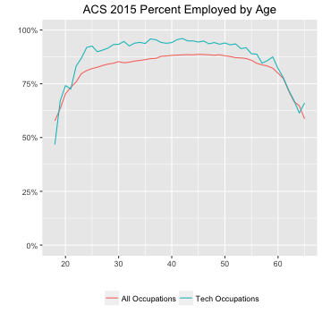
For nearly the entire working age population, tech workers are employed at substantially higher rates than workers in other occupations. If employability is hard to maintain for older workers in tech, it is even moreso in other occupations. This suggests that workers in tech, given the high demand of the occupation itself, are more insulated from employment fluctuations or ageism than other occupations.

Full-time year-round status by age

For our income assessments above we have been focusing on full-time, year-round workers to ensure that all respondent’s income measures are comparable. However this might be hiding a bias if older workers are not as represented in this group as younger ones. In other words, for each age we would like to see what proportion are working full-time and year-round. Whereas we can refer to the previous section as a measure of employability, here we consider a measure of under-employment.

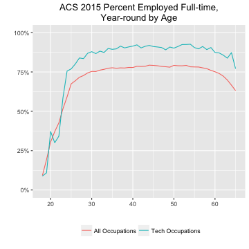
Among employed workers 18-65 in all occupations, 71% worked full-time and year-round in the prior 12 months. For those in tech occupations, 86% were working full-time and year-round. To me this is quite an interesting finding. Tech workers remain employed full-time at very high rates throughout all stages of their career. As someone well into his mid-career stage, to me this encouraging result suggests that tech can be a bit of a safe haven for us old-timers. For comparison among the professions we examined earlier, the full-time year-round employment rate for lawyers was 88%, and for doctors was 83%.

Tangentially, this touches upon another debate that frequently surfaces regarding tech occupations: that salaries are kept artificially low by collusion, market manipulation, visa programs, legislation and other tactics. These findings suggest that aggregate demand for tech workers is very high, as high or higher than other professions at the top end of the income scale. Yet, tech salaries are well below these professions. Although well beyond the scope of the present work, it may be possible to use ACS data to construct robust measures of aggregate occupational demand and explore why tech salaries appear to be low in comparison to other occupations that have similarly high levels of demand.

Age and industry

The last hypothesis we will consider in this analysis is whether age is a factor in the tech industry rather than tech occupations. The IND variable records the Census Bureau’s classification of each respondent’s self-reported industry. Again, since these codes were designed to broadly cover all aspects of the economy, there is some interpretation involved in determining what we would consider belonging to the “tech industry”.

IND Code	Unweighted count	Weighted count	Label
6490	1,647	167,285	Software publishing
6672	1,215	126,647	Internet publishing and broadcasting and web search portals
6680	6,899	713,569	Wired telecommunications carriers
6690	3,621	394,587	Telecommunications, except wired telecommunications carriers
6695	1,845	185,192	Data processing, hosting, and related services
6780	575	57,209	Other information services
7380	25,288	2,625,530	Computer systems design and related services
7390	20,297	1,994,390	Management, scientific, and technical consulting services
7460	7,543	722,397	Scientific research and development services

This table includes the 9 industry codes that will be used in this analysis to comprise “the tech industry”. The weighted population count of workers in these industries is 6,986,806, 3.7% of the population 16 and over.

The intersection between our tech occupations and tech industry classifications is significant, lending some face validity to our choices. Of all tech industry workers, 27% work in technical occupations, compared to just 1% for all other industries. In addition, of workers in tech occupations, 41% are employed in the tech industry, compared to 3% of workers in non-technical occupations. The table below shows the full age distribution for each of the 9 tech industries identified above.

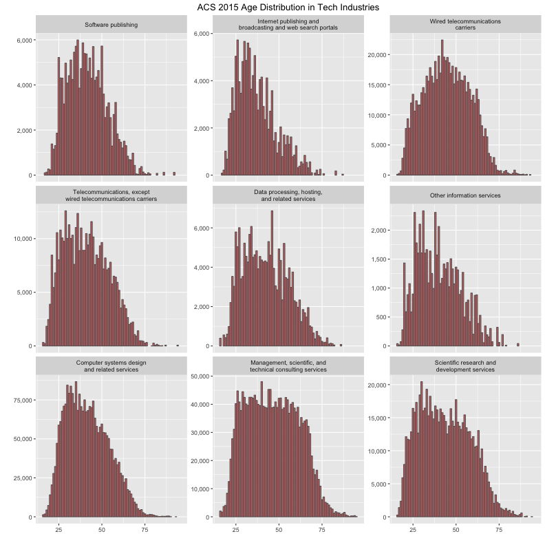
The median age is 40 or above in all these industries except for “Other information services” in which it is 39, and “Internet publishing” in which it is just 35. Whipper-snappers! On the other end of the spectrum, “Management, scientific, and technical consulting services” has the highest median age, at 46.

Now let’s examine the intersection of tech occupations and tech industries by looking at four more age distributions. In the top row are non-technical occupations, while the bottom row are workers in tech occupations. The left column are non-tech industries, while the right column are workers in tech industries.

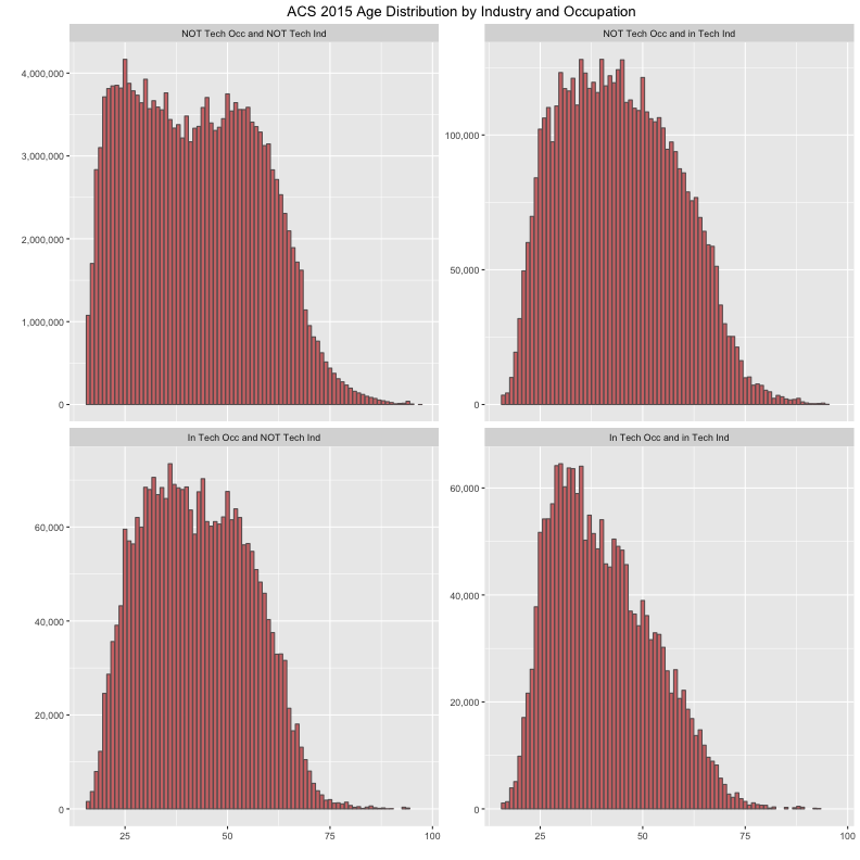
In the top left, we have the age distribution for workers in non-technical occupations working in non-technical industries. The median age here is 42. In the bottom right is the age distribution for workers in technical occupations working in technical industries, and the median age is 39. Although the median ages are not very different, it is clear from the shape of the distributions tech workers in tech industries skew younger. In the top left, 35% of workers are 50 or above, whereas in the bottom right, only 24% of workers in tech occupations and tech industries are 50 or over.

Concluding Remarks

The American Community Survey is a veritable treasure trove of valuable information for researchers interested in all manner of demographic questions about the US population. This analysis has barely scratched the surface of the depth in this valuable dataset. Here, we’ve only made use of 8 variables in 1 sample. There are hundreds of additional variables collected in the ACS in addition to over 15 years of individual samples. The Census Bureau periodically creates special 3-year and 5-year PUMS datasets by combining the individual year datasets together along with providing more detailed geographic coding. These can be especially useful when examining smaller subsets of the population. For instance, our intersection of tech workers in tech occupations has an unweighted case count of 17,949. While sufficient for top-level analyses, if one were interested in further segmenting this group—by education or geography—then it may make sense to turn to the larger 3- or 5-year samples. Finally, the IPUMS project makes analysis of the ACS extremely easy. Anyone can create an account, select the variables and samples they are interested in, and be working on an extract of the ACS data in a matter of minutes.

As promised, all the code used in this analysis is available in this R script: acs2015_age-and-tech.R.txt. The approach I have used is to load the ACS extract into a PostgreSQL database. Years ago I wrote this small python script for this purpose and it still works for all IPUMS extracts. Alternatively, you can use the ACS dataset to extract a CSV and use R’s read.csv function to import as an R data frame.