Adventures in Numerical Analysis
The best tools let you focus on your work rather than on the limitations of the tool itself. This is a fairly common metric when comparing the suitability of programming languages or libraries—the best ones to use are those that “get out of your way” and allow you to direct your thoughts and attention to the problem domain. You want to be able to think in pure terms, “How do I solve X?”, instead of the tainted “How do I solve X with Y?”
In numerical methods it is often not possible to ignore the limitations of the tools, especially when the tool is something as basic as floating point representation. A great deal of care needs to be taken to ensure that the implementation of a numerical algorithm will be accurate despite the limits of machine precision. If instead you try to think purely in terms of the algorithm, your results may not be what you expect. The constraints of the floating point representation of Real numbers cannot be ignored.
I recently relearned this lesson when adapting an algorithm for calculating the Normal Quantile function in Python. Wichura’s 1988 algorithm AS241 uses parameters from a 7-term polynomial approximation of the inverse cumulative normal distribution to generate normal deviates corresponding to a given lower-tail probability with error on the order of 1e-16. This is essentially the limit of machine precision available with a 64-bit floating point representation. In the original Fortran algorithm for function PPND16, Wichura writes the multiplication of the terms in reverse order so that the only operations are multiplication and addition:
    PPND16 = Q * (((((((A7 * R + A6) * R + A5) * R + A4) * R + A3)
 *             * R + A2) * R + A1) * R + A0) /
 *             (((((((B7 * R + B6) * R + B5) * R + B4) * R + B3)
 *             * R + B2) * R + B1) * R + ONE)
    RETURN
Translated literally into Python with A and B as lists of length 8 containing the parameters, I started with this:
result = Q * (((((((A[7] * R + A[6]) * R + A[5]) * R + A[4]) * R + A[3]) *  \
            R + A[2]) * R + A[1]) * R + A[0]) /                             \
            (((((((B[7] * R + B[6]) * R + B[5]) * R + B[4]) * R + B[3]) *   \
            R + B[2]) * R + B[1]) * R + 1.0)
return result
I verified that the results from my Python implementation matched
exactly what is produced by the qnorm function in R, which
uses a C version of Wichura’s algorithm and is certainly peer-reviewed
enough to be considered authoritative. I could have stopped there, but
looking at the above code I really wanted to clean it up. I mean, look
at it, it’s ugly! Since I was implementing this algorithm in Python, why
not make it more Pythonic? A couple of list comprehensions will
make that jumbled mess look a lot nicer:
result = Q * sum([a * pow(R, i) for i, a in enumerate(A)]) /
             sum([b * pow(R, i) for i, b in enumerate(B)])
There is perhaps a more clever way of doing this using
reduce and operator.mul, but even this is a
welcome improvement, aesthetically at any rate, over the original
Fortran.
Note that these are algebraically equivalent forms of the two
summations. In both the numerator and denominator, there are 8 terms
(including a constant) and the result is the sum of the ith term of
A (or B) multiplied by R raised
to the ith power. Unfortunately, the aesthetically-pleasing Pythonic
calculation is not numerically equivalent: there are small, systematic
error perturbations across the range of possible inputs.
Using the rpy2 module I am validating my custom Z-quantile function
against the qnorm function of R, at 1000 p-values ranging
from 0.001 to 0.999:
    import rpy2, rpy2.robjects
    P = range(1, 1000)
    for p in P:
        p /= 1000.0
        rpy2.robjects.r.assign('p', p)
        rpy2.robjects.r('z <- qnorm(p)')
        z = rpy2.robjects.r('z')
        print p, "\t", "{:.20f}".format(quantile_z(p) - z[0])
Whereas the first translation of the algorithm—the ugly one that is
faithful to the Fortran original—produces results that are binary exact
matches to R’s qnorm, the Pythonic version introduces small
errors that exhibit an interesting pattern. Here is a tabulation of
those error values:
Value           Count      Pct
=====           =====      ===
-8.8818e-16       3       0.30%
-6.6613e-16       8       0.80%
-4.4409e-16      32       3.20%
-3.3307e-16      12       1.20%
-2.2204e-16      85       8.51%
-1.6653e-16       5       0.50%
-1.1102e-16      85       8.51%
-8.327e-17        2       0.20%
-5.551e-17       45       4.50%
-4.163e-17        1       0.10%
-2.776e-17       20       2.00%
-2.082e-17        1       0.10%
-1.388e-17       14       1.40%
-6.94e-18         8       0.80%
-5.2e-18          2       0.20%
-3.47e-18         3       0.30%
-1.73e-18         2       0.20%
-8.7e-19          1       0.10%
0.0             345      34.53%
8.7e-19           1       0.10%
1.73e-18          2       0.20%
3.47e-18          3       0.30%
5.2e-18           2       0.20%
6.94e-18          8       0.80%
1.388e-17        12       1.20%
2.082e-17         1       0.10%
2.776e-17        20       2.00%
5.551e-17        56       5.61%
8.327e-17         3       0.30%
1.1102e-16       80       8.01%
1.6653e-16        1       0.10%
2.2204e-16       87       8.71%
3.3307e-16       11       1.10%
3.8858e-16        1       0.10%
4.4409e-16       26       2.60%
6.6613e-16        7       0.70%
8.8818e-16        4       0.40%
A plot of the error values against p reveals the systematic pattern:
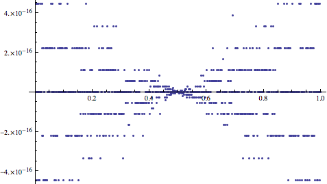
Wild, isn’t it? The magnitude of the errors is very small, below 1e-15, but the fact that a systematic pattern emerges is a dangerous signal. Even though they are unlikely to cause problems in isolation, it is unclear how these error perturbations may perpetuate and manifest greater discrepancies at a large scale. To be safe, we should stick to the faithful, if ugly, translation of the original algorithm in order to ensure that our results match certified accepted values.
In Wichura’s original 1988 paper he notes,
Evaluation of the polynomials A-F involves the addition and multiplication only of positive values; this enhances the numerical stability of the routines.
Clearly there was a reason he explicitly used the ugly expansion of
the polynomials in the original code: there can be subtle errors in
floating-point arithmetic when using alternate formulations even though
they are algebraically equivalent. The Pythonic expression uses the
pow() function to raise each term to its corresponding
power in the series and this method produces different round-off
characteristics than Wichura’s method wherein the terms are expanded out
from right to left. Wichura must have recognized that exponentiating the
r terms is a less numerically stable calculation.
This exercise confirms why so many numerical algorithms use seriously old-school Fortran code that has been unaltered for 50 years. Once a numerical method is certified, there is an inherent danger in twiddling with its inner mechanics. Porting methods to a new language itself takes a great deal of care. Fortunately, Fortran, C, Python, and others rely on the same underlying IEEE 754 Standard for Floating-Point representation of Real numbers. This is why my first—faithful—translation from Fortran to Python matches the R Project’s faithful translation to C. My vain efforts to adapt the method to be more Pythonic turned out not to be such a good idea. As in the old saying about premature optimization, it is far better to be right than to be clever.